


In Part 1, I looked at how files such as CSV and TSV move into Snowflake.
But not all data arrives in neat rows and columns.
APIs and modern applications often return JSON. At first, JSON can look like a confusing mixture of brackets, labels, lists and information nested inside other information.
The ideas that helped me understand it were:
JSON → VARIANT → Path Notation → Arrays → FLATTEN → Cast → Analyse
Once I understood what each stage was doing, working with semi-structured data became much less intimidating.
1. Think of nested JSON like Russian dolls
A simple JSON object might look like this:
{
  "name": "Fiona",
  "country": "UK"
}
That is fairly easy to read.
But JSON can also contain information inside other information.
For example, a tweet might contain something like:
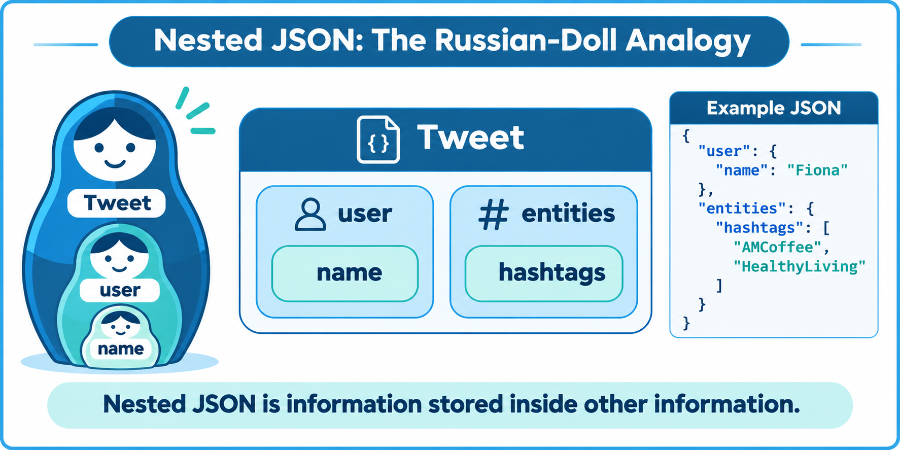
Tweet
├── user
│   └── name
└── entities
    └── hashtags
This is where I found the Russian-doll analogy useful.
Imagine the outside doll represents the whole tweet.
Inside it, there may be another section called user.
Inside user, there may be another value called name.
So to reach the person's name, we keep opening the layers:
Tweet → user → name
The same idea works for:
Tweet → entities → hashtags
The important thing is that we do not need to understand the whole JSON document at once.
We only need to work out:
What path do I need to follow to reach the value I want?
2. VARIANT gives Snowflake somewhere to store the JSON
Before we can explore JSON, Snowflake needs somewhere to keep it.
This is where the VARIANT datatype becomes useful.
For example:
RAW_STATUS VARIANTI think of VARIANT as:
A flexible container that can hold the original JSON structure.
With traditional structured data, we might immediately create columns such as:
NAME
COUNTRY
DATE
STATUS
JSON is different because it may contain nested objects, arrays and many fields that we do not yet know whether we need.
Instead of forcing everything into columns immediately, we can first store the complete JSON object inside a VARIANT column.
That gives us the flexibility to decide later which parts of the JSON are useful.
For example, one row in a table might contain an entire tweet inside RAW_STATUS.
Snowflake keeps the structure, and we can then navigate through it.
3. Path notation lets us move through JSON
Once the JSON is stored, we need a way to retrieve individual values.
Snowflake uses path notation.
For example:
RAW_STATUS:user:nameI read this from left to right:
Start with RAW_STATUS → go inside user → retrieve name.
Another example is:
RAW_STATUS:entities:hashtagswhich means:
Start with the tweet → go into entities → find hashtags.
This was one of the biggest turning points for me when learning JSON.
Instead of staring at a large JSON object, I could treat it almost like following directions:
Start here
   ↓
Go inside this section
   ↓
Go inside the next section
   ↓
Find the value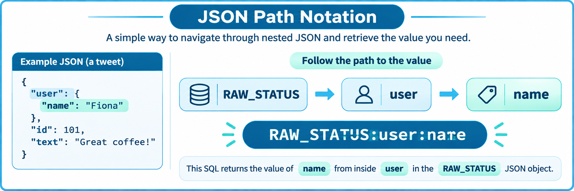
4. What is an array?
JSON can also contain arrays.
An array is simply a list of values or objects.
For example, a tweet could contain:
["AMCoffee", "HeartThis", "HealthyLiving"]All three hashtags belong to the same tweet.
If I only wanted the first hashtag, I could use:
RAW_STATUS:entities:hashtags[0]The [0] means:
Give me the first item in the array.
This is because programming languages normally start counting list positions at zero.
So:
[0] = first item
[1] = second item
[2] = third item
But there is an obvious problem.
What if I do not want just the first hashtag?
What if I want to analyse every hashtag?
That is where FLATTEN becomes useful.
5. FLATTEN turns an array into rows
Imagine one tweet contains this array:
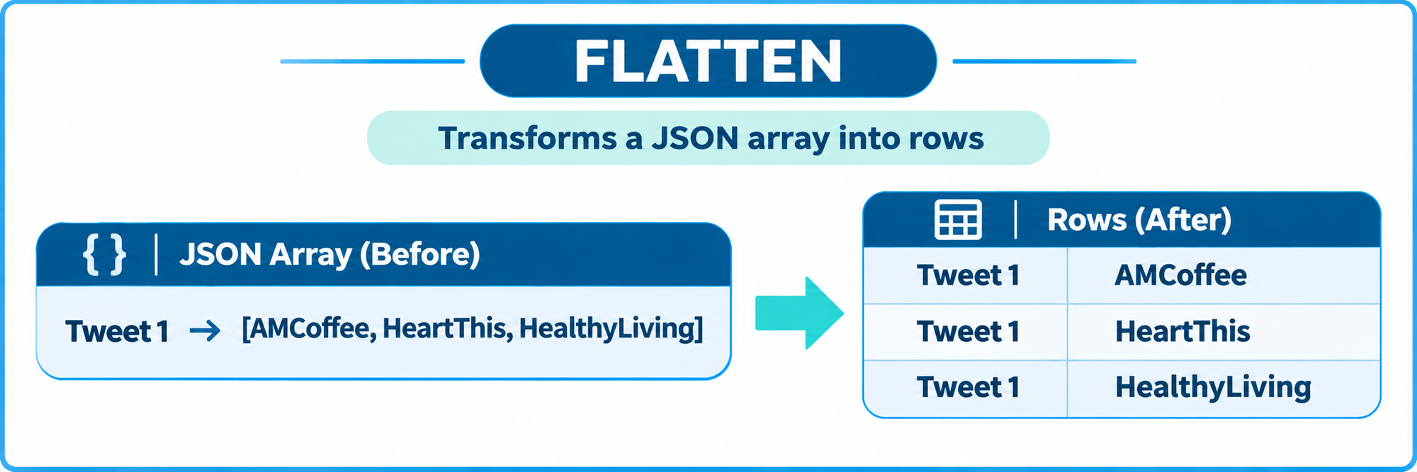
["AMCoffee", "HeartThis", "HealthyLiving"]Before using FLATTEN, Snowflake effectively sees:
Tweet 1 → [AMCoffee, HeartThis, HealthyLiving]The three hashtags are stored together inside one array.
For analysis, it would often be much more useful to have:
Tweet 1 → AMCoffee
Tweet 1 → HeartThis
Tweet 1 → HealthyLiving
That is what FLATTEN helps us do.
A simplified example looks like:
FLATTEN(
    INPUT => RAW_STATUS:entities:hashtags
)
I read this as:
Find the hashtags array and turn each item inside it into a separate row.
This is an important idea because SQL works naturally with rows.
Once those values become rows, we can:
- count them
- filter them
- group them
- compare them
- analyse them
- use them in dashboards
6. Why do we use LATERAL FLATTEN?
In the exercises, I used code such as:
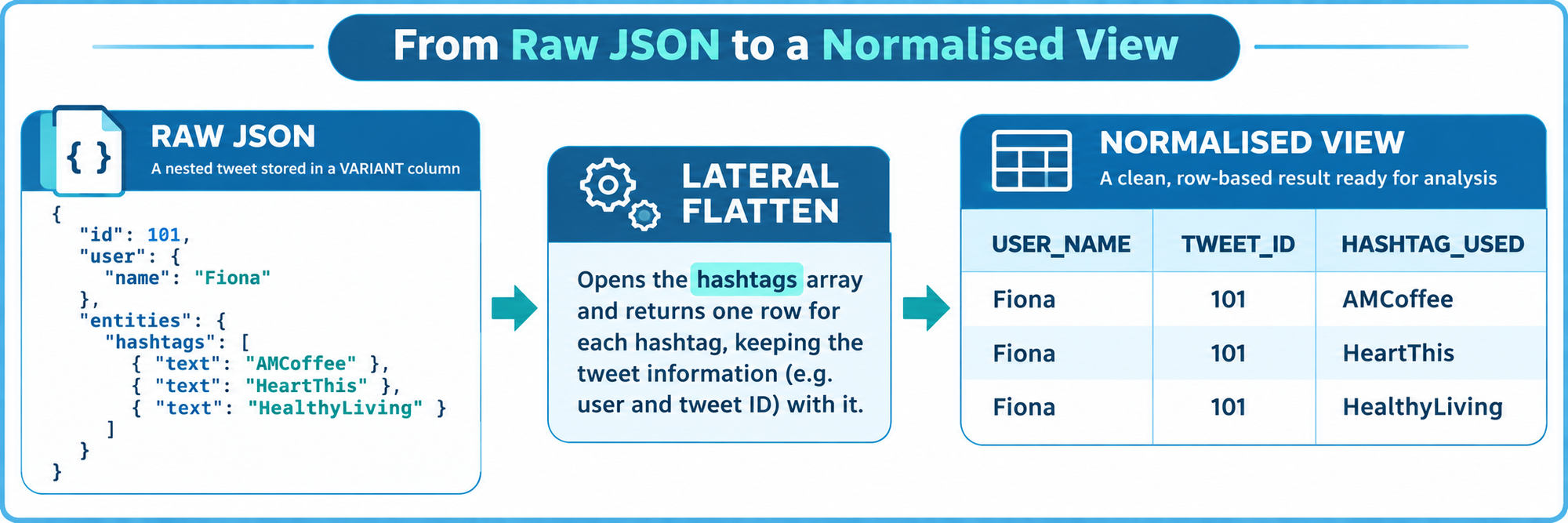
SELECT
    RAW_STATUS:user:name::text AS USER_NAME,
    RAW_STATUS:id AS TWEET_ID,
    VALUE:text::varchar AS HASHTAG_USED
FROM TWEET_INGEST,
LATERAL FLATTEN(
    INPUT => RAW_STATUS:entities:hashtags
);
There are a few things happening here.
First:
RAW_STATUS:user:name::textretrieves the user name.
Then:
RAW_STATUS:idretrieves the tweet ID.
Finally:
LATERAL FLATTEN(
    INPUT => RAW_STATUS:entities:hashtags
)
opens the hashtag array for the current tweet.
The word LATERAL initially looked complicated to me.
The way I now think about it is:
For each original row, look inside its array and return the items found there.
So we keep information from the original tweet, such as the user and tweet ID, while also creating one row for each hashtag.
The flattened item is available through a column called:
VALUESo:
VALUE:textmeans:
Take the current item produced byFLATTENand retrieve itstextvalue.
7. Casting converts JSON values into useful SQL types
When we retrieve a value from JSON, we may want Snowflake to treat it as a normal SQL datatype.
That is where casting comes in.
For example:
::textmeans:
Treat this value as text.
And:
::datemeans:
Treat this value as a date.
For example:
RAW_STATUS:created_at::datemeans:
Find created_at inside the JSON and convert it into a date.
Once Snowflake understands that value as a date, normal SQL operations become much easier.
We can sort by it:
ORDER BY RAW_STATUS:created_at::dateOr group the records by date:
SELECT
    RAW_STATUS:created_at::date AS TWEET_DATE,
    COUNT(*) AS TWEET_COUNT
FROM TWEET_INGEST
GROUP BY RAW_STATUS:created_at::date
ORDER BY TWEET_COUNT DESC;
This is where semi-structured JSON starts becoming familiar analytical data.
8. Views can hide some of the JSON complexity
After flattening the data, we can save the query as a view.
For example:
CREATE OR REPLACE VIEW HASHTAGS_NORMALIZED AS
SELECT
    RAW_STATUS:user:name::text AS USER_NAME,
    RAW_STATUS:id AS TWEET_ID,
    VALUE:text::varchar AS HASHTAG_USED
FROM TWEET_INGEST,
LATERAL FLATTEN(
    INPUT => RAW_STATUS:entities:hashtags
);
I think of a view as a saved query.
Instead of writing all of the JSON navigation and FLATTEN logic every time, I can simply query:
SELECT *
FROM HASHTAGS_NORMALIZED;
The underlying data is still JSON.
The view gives us a cleaner, more familiar table-like way of working with it.
This is useful because somebody analysing the data may not need to know how complicated the original JSON structure was.
9. The complete picture
The workflow I now use when thinking about JSON in Snowflake is:
JSON
  ↓
VARIANT
  ↓
Path Notation
  ↓
Find an Array
  ↓
FLATTEN
  ↓
Cast
  ↓
View / Analyse
Each step has a different job.
JSON
The original semi-structured data.
VARIANT
The flexible Snowflake datatype that stores it.
Path notation
Lets us navigate through the JSON.
Arrays
Hold lists of values or objects.
FLATTEN
Turns items inside an array into individual rows.
Casting
Turns JSON values into familiar SQL datatypes.
Views
Let us save the transformation logic and work with a cleaner representation.
The biggest lesson for me
The biggest lesson was that JSON does not need to be understood all at once.
At first, a large JSON object can look overwhelming.
But I now approach it one question at a time:
Where is the value I want?
Then:
What path gets me there?
Then:
Is the value inside an array?
If it is, I can use FLATTEN.
And finally:
What datatype do I want Snowflake to treat that value as?
That turns something that originally looked complicated into a repeatable process:
Store it → follow the path → flatten if needed → cast it → analyse it.
For me, that is the key to understanding semi-structured data in Snowflake.