


In Part 1, we diagnosed the problem with the Superstore flat file. In Part 2, we pulled that file apart into proper tables and saw how primary and foreign keys hold those tables together. Now, we’re going to take that structure one step further and turn it into something you’ll see constantly in analytics work: the star schema.
If you want to go back to part 1 or part 2, click on the images below:
Instead of just understanding why tables should be separated, we’re now shaping them into a structure that is easier to query, easier to explain, and much easier to use in tools like Tableau or Power BI.
What Is a Star Schema?
A star schema is a way of organizing your data model around two main types of tables: fact tables and dimension tables.
The fact table sits in the center of the model. This is where the measurable activity lives. In Superstore, that could be each order item, with fields like sales, quantity, discount, and profit. These are the numbers you want to add up, average, compare, or trend over time.
The dimension tables sit around the fact table and provide context. They describe the who, what, where, and when behind each row in the fact table. For example, a sale on its own does not tell you much. But sales by customer, product category, order date, or region suddenly become useful.
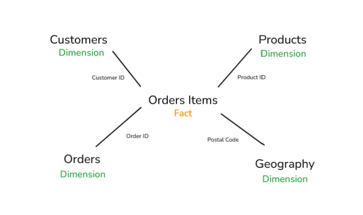
That is the key idea behind a star schema: the fact table tells you what happened, and the dimension tables help you understand who, what, where, and when it happened.
When you draw this out, the fact table sits in the middle with dimensions branching out around it. That’s where the name “star schema” comes from!
The Superstore Star Schema
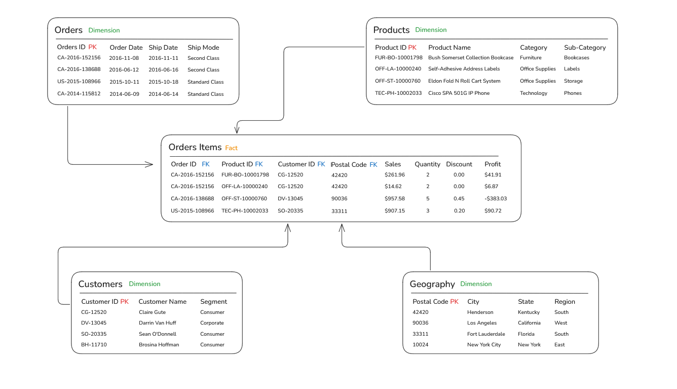
The fact table is Order Items. Each row represents one product sold within one order. It contains the measurable fields we want to analyze, such as Sales, Quantity, Discount, and Profit. It also contains the foreign keys that connect each row to the surrounding dimensions: Order ID, Customer ID, Product ID, and Postal Code.
The Customers dimension has one row per customer. Customer ID is the primary key. Descriptive customer information lives here, such as Customer Name and Segment. This lets us analyze measures like sales and profit by customer type.
The Products dimension has one row per product. Product ID is the primary key. Fields like Product Name, Category, and Sub-Category live here. This is the table you use when you want to understand what was sold.
The Orders dimension holds order-level context that is not a measurement. This includes fields like Order Date, Ship Date, and Ship Mode. It has one row per order, with Order ID as the primary key.
The Geography dimension holds location context. Postal Code is the primary key, and fields like City, State, and Region live here. Breaking Geography out separately is useful when you want to analyze location patterns independently from individual customers.
The important thing is that the Order Items fact table sits at the center, while each dimension gives that activity more meaning. Sales by itself is just a number. Sales by customer segment, product category, ship mode, and region becomes analysis.
Fact Tables and Grain
Now that we’ve identified Order Items as our fact table, there’s one important design decision worth slowing down for: its grain. In simple terms, grain means: what does one row represent?
In our Superstore model, the grain of the Order Items fact table is one product within one order. That is a deliberate choice. Each row answers the question:
“How much of this specific product was sold in this specific order?”
If we had chosen a coarser grain, such as one row per order, we would lose important detail. We could still analyze total sales by order, but we would not be able to properly analyze sales by product, category, or sub-category. Questions like “Which sub-category drove the most revenue last quarter?” would become much harder, because the product-level detail would already be collapsed.
If we chose a finer grain, such as one row per unit sold, the table would become much larger without adding much useful analytical value for most business questions.
Getting the grain right means thinking carefully about the questions your analysis needs to answer. The fact table should be detailed enough to support those questions, but not so detailed that it becomes unnecessarily large or awkward to use.
Writing Queries Against a Star Schema
Here’s where everything starts to come together.
Once your data is organized into a star schema, the SQL you write becomes much more consistent. Most analytical questions follow the same pattern:
Start with the fact table, join to the dimensions you need, group by the dimension fields you want to analyze, and aggregate the measures.
For example, if you want total sales by customer segment, you start from the Order Items fact table, join to the Customers dimension, and group by customer_name.

Notice the pattern.
The fact table is the starting point because that is where the measures live. In this case, sales comes from order_items.
The dimension table comes in through a join. Here, we join to customers so we can turn a customer_id into a readable customer name.
The measure is aggregated in the SELECT statement using SUM().
The dimension attribute appears in the GROUP BY, because that controls the level of detail in the result. Since we group by customer_name, the query returns one row per customer.
Once you understand this, querying a star schema becomes much easier. You are not learning a completely new structure every time. You are applying the same logic again and again: start with the facts, join the context, then aggregate the numbers.
The Payoff
Across this three-part series, we took one overwhelming flat file and turned it into something an analyst can actually work with.
In Part 1, we looked at why flat files break down: repeated data, update problems, and the challenge of cramming orders, customers, and products into a single row.
In Part 2, we pulled those entities apart, gave each one its own table, and learned how primary and foreign keys hold the structure together.
In Part 3, we formalized that structure into a star schema: a fact table at the center, dimensions surrounding it, and queries that follow a consistent, predictable pattern.
That progression, from messy flat file to clean analytical model, is what data modelling is really about. It is not just tidier spreadsheets. It is a way of thinking about data that scales as it grows, holds up as more people use it, and makes the analyst’s job genuinely easier.
Superstore is a practice dataset, but the pattern is real. The structure we built here is the same shape you will find at a SaaS company, a retail chain, or an e-commerce business. The table names may change and the measures may be different, but the thinking is the same.
Learn it once, and you will start recognizing it everywhere.
That’s a wrap on the three-part Data Modelling Series. Thanks for reading!