Granularity, Joins, and Schemas

Working with data in tools like Alteryx, Tableau Prep, or SQL is a powerful way to find insights. However, this power comes with a responsibility: ensuring your numbers are actually correct. We've all been there: you perform what looks like a simple join, and suddenly your row count explodes. Your SUM(Sales) is 10 times what it should be, and you're left staring at your flow wondering what went wrong.

The culprit, 99% of the time, is a mismatch in granularity.

In this blog post, we'll break down what granularity is and why it's the most important concept to master for accurate joins and analysis. We'll start with the fundamentals of identifying the level of granularity of a dataset, then explore the common pitfalls of joining tables with different granularities, and finally, see how this concept scales up to building robust database schemas.

What is Granularity?

Granularity, in simple terms, is the level of detail represented by a single row in your dataset. Think of it as the "scope" of each record.

• High Granularity (Fine-grained): This is highly detailed data. Each row represents a small, specific "thing" or "event."
  • Example: Individual sales transaction lines, individual web page clicks, or sensor readings per second.
• Low Granularity (Coarse-grained): This is aggregated or summarised data. Each row represents a larger, more general grouping.
  • Example: Total sales per store per day, average monthly website visitors, or regional profit targets.

The easiest way to identify the grain of any dataset is to ask one simple question:

"What does one row in this table represent?"

Let's look at two tables.

Table A: Sales Transactions (High Granularity) This table's grain is "one product line item per transaction."

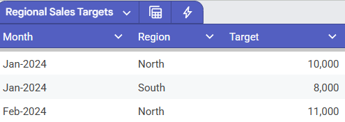
Table B: Regional Sales Targets (Low Granularity) This table's grain is "one sales target per region per month."

Both tables are valid and useful, but they describe the business at very different levels. The problems start when we try to combine them without thinking.

The Join Problem: When Granularities Collide

This is where most data-joining errors occur. Let's say we want to compare our sales performance (Table A) against our targets (Table B). The grain of Table B is [Month] and [Region].

A common mistake is to join them only on their common field, Region, and then try to filter by month later.

What happens? Let's say we have 500 sales transactions in the "North" region that all occurred in January (from Table A). When we join to Table B on Region = "North":

• The "North" target of 10,000 for "Jan-2024" will be duplicated 500 times—once for every single "North" transaction in January.
• The "North" target of 11,000 for "Feb-2024" will also be duplicated 500 times!

The result is a table that is completely unusable. This "fan-out" creates massive, incorrect numbers.

The Solution: Aggregate Before You Join

To fix this, you must make the granularity of your datasets match before you perform the join.

The grain of our target table (Table B) is [Month] and [Region]. Therefore, we must aggregate our Sales_Transactions table (Table A) to that exact same level.

1. Prep Table A: First, you'll need to create a Month column from the Transaction_Date field (e.g., "Jan-2024").
2. Aggregate Sales: Use an Aggregate tool or step.
   • Group by: Month and Region.
   • Summarise: SUM(Amount).
3. Join: The output of this aggregation is a new table where the grain is "total sales per region per month." Now this table has the exact same grain as Table B. You can join them cleanly on two keys: Month AND Region.

The result will be a clean, 1-to-1 join, and your numbers will be correct.

Granularity in Schemas

While fixing a two-table join is a common task, this same concept is the foundation of professional data warehousing, most famously in the star schema.

A star schema is a data model designed to manage different granularities. It consists of:

• One Fact Table: This table is at the center and contains the highest-granularity data (the "facts" or "measurements," like Sales_Amount, Quantity_Sold). Its grain is usually "one event."
• Multiple Dimension Tables: These tables surround the fact table. They contain the descriptive, lower-granularity attributes (the "who, what, when, where," like Product_Name, Store_Address, Customer_Name). The grain of a Dim_Product table is "one product."

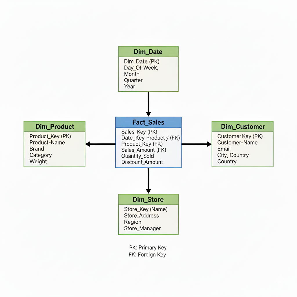
In this model, you join a low-granularity dimension (like Dim_Product) to the high-granularity fact table (Fact_Sales) on a Product_ID key. This one-to-many join is intentional and correct. You are intentionally enriching your high-granularity facts with their low-granularity descriptions.

The schema works because the relationships are clearly defined, and all descriptive context (dimensions) relates back to the central event (fact).

Tips and Best Practices

• Always Ask "The Question": Before any join, stop and ask: "What does one row represent in Table A? What does one row represent in Table B?"
• Beware the Many-to-Many: If the answer to the above question doesn't result in a clean one-to-one or one-to-many join (from dimension-to-fact), you are likely creating a fan-out.
• Aggregate is Your Friend: Use aggregation to "roll up" your fine-grained data to a coarser grain that matches your other tables.
• Document Your Grain: When you build a complex workflow, leave a comment or annotation specifying the grain of the data at crucial points. Your future self will thank you.

Conclusion

Understanding granularity isn't just a technical exercise; it's the fundamental skill that ensures the integrity of your analysis. It's the difference between a dashboard that reports 5,000,000 in "target sales" and one that correctly reports 10,000.

By mastering this concept, you move from simply joining data to designing robust, accurate, and insightful data models that stakeholders can trust.