From Raw Data to Insights: Building a Data Pipeline with Snowflake and SQL

From Data Storage to SQL

In a previous blog, The Data Journey: Where Data Lives, we explored the different places data can be stored, from flat files and databases to data warehouses and modern data lakehouses.

But once our data has a place to live, how do we actually interact with it?

One platform that allows us to store and work with data is Snowflake, a cloud-based data platform designed to store, process, and analyze large amounts of data.

To interact with the data stored in Snowflake, we use Structured Query Language (SQL), a programming language that allows us to retrieve, manage, and transform data within databases.

SQL is a powerful language with several types of statements, but for this project, we'll focus on two important categories:

• Data Definition Language (DDL): Used to define and manage database structures, such as creating tables with CREATE TABLE or modifying existing ones with ALTER TABLE. In simpler terms, DDL focuses on how the data is structured and stored.
• Data Manipulation Language (DML): Used to manage the data within those tables, including inserting records with INSERT, updating values with UPDATE, and removing records with DELETE. In simpler terms, DML focuses on making changes to the data itself.

Together, these commands allow us to organize and prepare data for analysis.

This past week, I had the opportunity to put these concepts to work by building a data pipeline using Python, Snowflake, SQL, and Tableau. Using NFL player statistics from the 2020–2025 seasons, I worked through the process of extracting raw data, transforming it into a structured relational model, and making it available for analysis in Tableau.

Let's walk through the process of how it all came together!

Extract: Collecting the Data

The first step in building my data pipeline was extracting the data I would be working with. For this project, I decided to use NFL statistics sourced from the nflverse GitHub repository.

Using Python in Google Colab, I created a script that utilized the nflreadpy library to retrieve two datasets:

• load_player_stats(): Weekly player statistics, including passing, rushing, receiving, defensive statistics, and more.
• load_team_stats(): Team-level statistics covering performance across games and seasons.

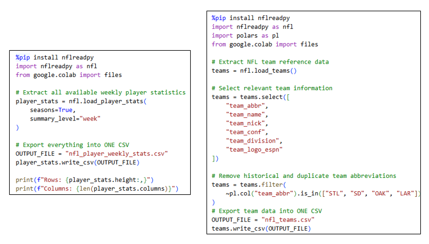
With access to historical NFL data, my goal was to focus on the 2020–2025 seasons and organize the information into a structured dataset that could support different types of analysis.

Once extracted, I exported the datasets into two separate CSV files and imported them into Snowflake, where I could begin exploring and transforming the data using SQL.

Transform: Preparing and Structuring the Data

Once the data was imported into Snowflake, I began exploring the raw dataset to better understand what I was working with. The original player statistics dataset contained 480,608 rows and 150 columns, with historical NFL statistics dating back to 1999.

While this provided plenty of information to work with, I wanted to narrow the scope of my analysis to the 2020–2025 seasons.

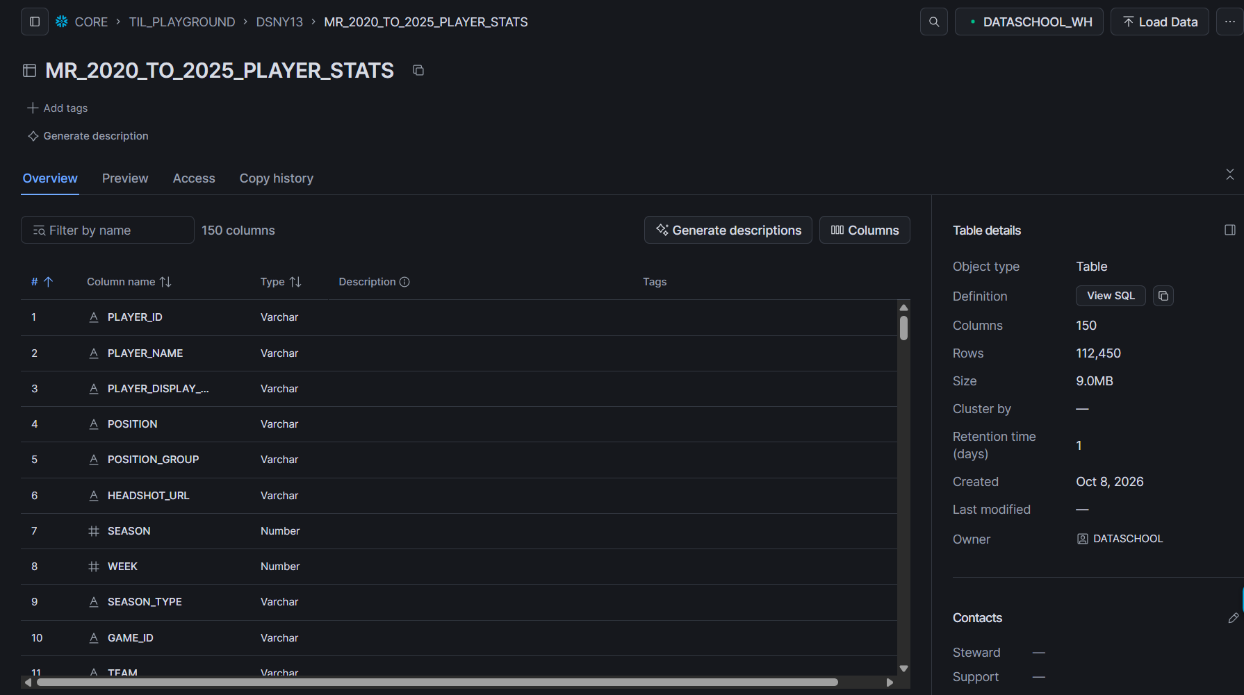
Using SQL, I created a new table with a CREATE TABLE AS SELECT statement, filtering the original dataset with a WHERE clause to include only the six seasons I wanted. This is also an example of the DDL statements we discussed earlier!

The resulting table contained 112,450 rows and 150 columns, giving me a more manageable dataset to start querying.

Understanding the Users

With my data narrowed down, the next question was: Who would actually be using this data, and what would they want to analyze?

For this project, I identified three potential users, each with different needs, and developed user stories to better understand what each would want to accomplish:

• Player Performance Analyst: Interested in tracking individual player performance over time and comparing players across positions.
• Team Performance Analyst: Focused on team performance, including conference and division comparisons and home versus away statistics.
• Game Analysis Specialist: Interested in analyzing individual matchups and understanding player contributions within specific games.

Designing and Building the Schema

With my users and their analytical needs identified, I could begin designing a relational data model that would support their different use cases.

Rather than keeping all the information in one large table, I decided to separate the data into fact and dimension tables.

In simple terms, fact tables contain measurable information, such as passing yards or touchdowns, while dimension tables provide descriptive information, such as player names, teams, and game details.

My final schema consisted of a central player-game fact table, six specialized statistical fact tables (Passing, Rushing, Receiving, Defense, Kicking, and Punt/Return), and three dimension tables (Player, Game, and Team).

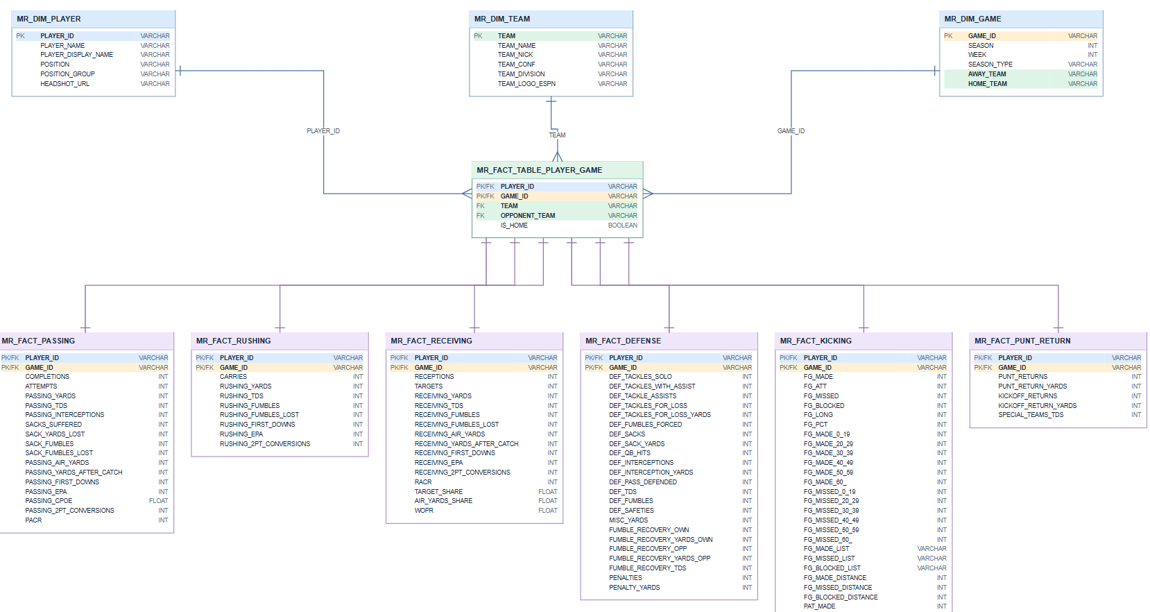
With the schema designed, I used SQL in Snowflake to create the individual tables. This involved using CREATE TABLE AS SELECT statements, along withCASE, CAST, and QUALIFY to organize and transform the data.

Below are a few examples of the SQL statements I used to create the tables within my schema.

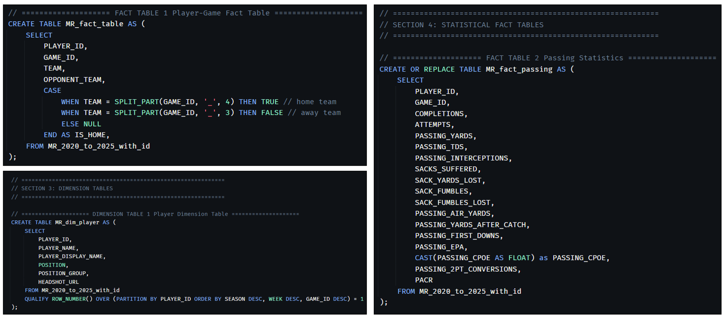
One of the biggest challenges throughout this process was determining how all these tables should be structured and connected. Once I had a clear schema in mind, writing the SQL to build the individual tables became much more straightforward.

Load: Connecting the Data to Tableau

With my fact and dimension tables created in Snowflake, the final step was making the data available for analysis.

Using Tableau's Snowflake connector, I connected directly to Snowflake and brought in the newly created tables. From there, I established relationships between the tables using shared identifiers such as PLAYER_ID, GAME_ID, and TEAM.

Rather than joining the tables directly in Snowflake, I used Tableau's logical data model to establish these relationships, allowing the tables to remain separate while still supporting analysis across the different datasets.

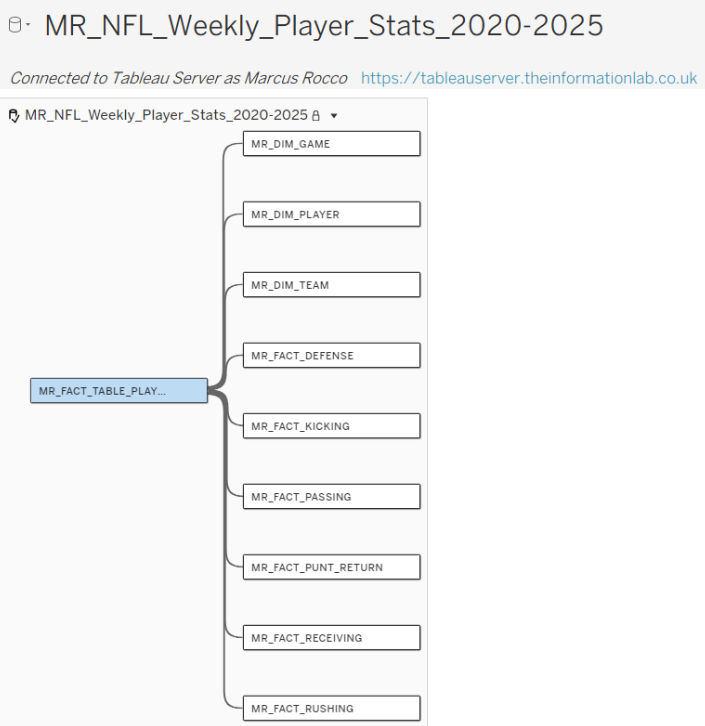
Once the relationships were established, I published the completed data model as a reusable data source to Tableau Server, enabling users to connect to and analyze the NFL statistics based on their individual needs.

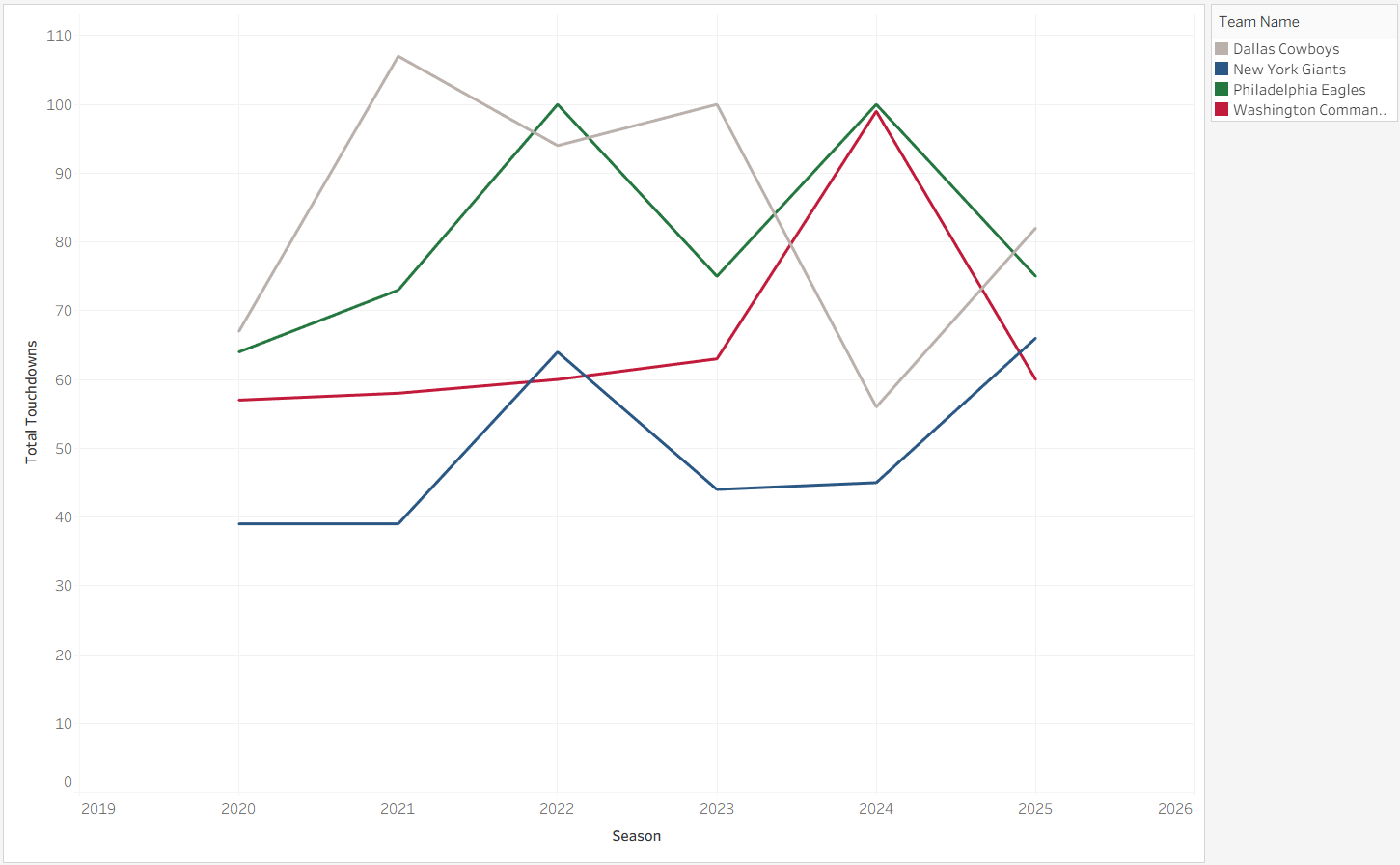
To validate that everything was working as expected, I created a simple visualization comparing the total touchdowns of NFC East teams across the 2020–2025 seasons. This allowed me to test the relationships and confirm that the data could be used to analyze trends across multiple seasons.

Final Thoughts & Takeaways

This project gave me the opportunity to revisit my coding background and build on the skills I developed throughout my education and previous work experiences. I also gained valuable hands-on experience in data engineering, working through the entire pipeline from extracting raw data to transforming it in Snowflake and making it available for analysis in Tableau.

One of my biggest takeaways was understanding just how important schema design is when working with large datasets. Taking the time to explore the data and consider the needs of different users made the transformation process much easier to approach.

Ultimately, this project helped me better understand how Python, Snowflake, SQL, and Tableau can work together to turn raw data into something structured, accessible, and ready for analysis.

Thanks for reading, and I hope you learned something new about Snowflake, SQL, and the process of building a data pipeline! Hopefully, this walkthrough has also inspired you to explore how you could build a data pipeline of your own!