


Principal component analysis and k-means clustering can be powerful tools in player recruitment, identifying similar players in order to narrow down the scouting pool. I used data from the 2017/18 season to try and identify potential replacements for Mousa Dembélé of tottenham. I searched for U23 players in the top 5 European leagues that have a similar skillset using pca and k-means cluster analysis.
Principal component analysis
What is principal component analysis?
PCA aims to reduce a larger set of individual variables (progressive passes, tackles won, take ons won % etc) into broader dimensions which are common to those variables.
When you perform a principal component analysis, you will get several principal components output. Each principal component is a linear combination of the original variables, and the coefficients of this linear combination are called loadings. The loadings represent the degree to which each variable contributes to that particular principal component.
In other words, PC1 and PC2 are new variables that are created by combining the original variables in a specific way. PC1 captures the largest amount of variation in the data, and the direction of the PC1 axis is the direction of greatest variance in the data. PC2 captures the second-largest amount of variation, and is orthogonal (perpendicular) to PC1, meaning that it captures a different pattern of variation in the data.
Typically, you could describe a massive data set with 2 to 3 principal components, accounting for ~90% of the variance within the data set.
In this case, due to the wide position filters I had, PC1 and 2 only explains 53% of the variance within this dataset. I will talk about the limitiations of this data further on.

To illustrate how this is calculated, let's look at Mousa Dembélé. He has a pc1 of -1.806867
This is calculated by multiplying each PC loading with the original (scaled) value of our metrics. So, from the report of our pca below, Dembele’s would be calculated as such:
(scaled number of times fouled) * 0.180194 (pc1 of fouled)
(scaled number of times dispossessed) * 0.4169 (pc1 of dispossessed)
(scaled number of interceptions) * -0.46906 (pc1 of interceptions)
(scaled passing %) * -0.412536 (pc1 of passing %)
(scaled number of progressive passes) * -0.300755 (pc1 of progressive passes)
(scaled number of tackles won) * - 0.358402 (pc1 of tackles won)
(scaled number of Take ons won) * 0.33151 (pc1 of take ons won)
(scaled take ons won %) * -0.272403 (pc1 of take ons won %)
= -1.806867
The same is done for each player and repeated for PC2.
Figures are scaled using z-scores where
Z = (observed value - mean of sample)/standard deviation of sample
This normalises the metrics so one having a larger scale doesn’t disproportionately affect results.
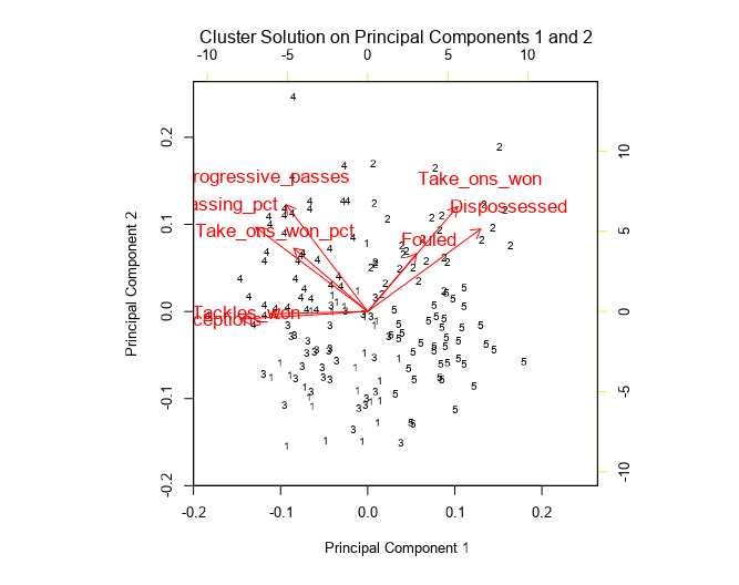
So, for the Mousa Dembélé case study, the biplot of pc1 and pc2 looks like this:

Where each number represents a player. The arrow's direction shows how much that factor influences the principal component.
The angle of the vectors (or loadings) can tell us how each factor is correlated.
When two vectors are close, forming a small angle, the two variables they represent are positively correlated. Example: Fouled and take ons won.
If they meet each other at 90°, they are not likely to be correlated. Example: Progressive passes and dispossessed.
When they diverge and form a large angle (close to 180°), they are negatively correlated. Example: take ons won and tackles.
Players with a high score in pc1 are likely to have high figures for take ons won, dispossessed and fouled. Those with a negative pc1 are likely to have larger numbers of tackles and interceptions.
Those with a high score in pc2 are likely to have higher numbers in progressive passes, pass completion % and take ons won %.
One limitation of the dataset used was the fact that position labels were not specific, so midfield includes many wingers and more attacking players, which introduces a lot more variance in terms of the take ons and fouled figures. A more specific set of filters would improve results.
K Means Cluster analysis
This is then used in tandem with k-means clustering. Cluster analysis is an unsupervised machine learning method. Put simply, this method aims to classify players into separate groups based on the multiple variables entered into the analysis. Players who are highly similar to each other are classified more closely than those who are highly dissimilar. K-means clustering seeks to minimise the within group variance whilst maximising the between group variance.
A centroid refers to the centre point of a cluster. It is calculated as the mean of all the data points assigned to a particular cluster.
In Alteryx, the k-means clustering tool is available in the Predictive Group of tools. It takes in a dataset and requires the user to specify the number of clusters (k) to create. Here's how it works:
Initialization: The algorithm starts by randomly selecting k data points from the dataset to serve as the initial centroids of the k clusters.
Assignment: Each data point is then assigned to the cluster whose centroid is closest to it in terms of Euclidean distance.
Recalculation: The centroids of each cluster are recalculated based on the mean of all the data points assigned to it.
Reassignment: The algorithm iterates between steps 2 and 3 until convergence is reached, which is defined as when the assignments of data points to clusters no longer change.
Output: Once the algorithm converges, the final cluster assignments and centroids are outputted as a new data set, where each data point is labelled with its assigned cluster.
Euclidean distance:
Euclidean distance is a measure of the distance between two points. It is the shortest distance between two points in a straight line. In two dimensions, it is the length of the hypotenuse of a right triangle formed by the two points and the origin. In three dimensions, it is the distance between two points in space.
The formula for calculating the Euclidean distance between two points (x1, y1) and (x2, y2) in a two-dimensional space is:
d = sqrt((x2 - x1)^2 + (y2 - y1)^2)
where sqrt is the square root function.
In general, the formula for the Euclidean distance between two points in n-dimensional space is:
d = sqrt((x2 - x1)^2 + (y2 - y1)^2 + ... + (zn - zn-1)^2)
where x1, y1, z1, ..., xn, yn, zn are the coordinates of the two points in n-dimensional space.
The Euclidean distance is commonly used in machine learning and data analysis, particularly in clustering algorithms such as k-means. It is used to measure the similarity or dissimilarity between two data points or observations, based on their coordinates or features. The smaller the distance, the more similar the data points are, and vice versa.
In summary, k-means clustering in Alteryx is a powerful tool for finding structure in unlabeled data by grouping similar data points together into clusters. The algorithm iteratively assigns data points to the nearest centroid, recalculates the centroids, and repeats until convergence is reached.
This means that the algorithm has reached a point where the assignments of data points to clusters no longer change. Specifically, convergence is achieved when the centroids of the clusters no longer move, meaning that they remain the same after the recalculation step.
When the algorithm converges, it means that it has found a stable solution that minimises the sum of squared distances between each data point and its assigned cluster's centroid. At this point, the clustering process is complete, and the final cluster assignments and centroids can be outputted as the results.
Going to back to our case study, the output of our k-means clustering is as follows:
We get some information about each cluster, showing that respective cluster’s correlation with each respective variable.
We also get a biplot where we have each player in their respective cluster plotted against principal components 1 and 2. In the previous example, each player was plotted as their own number, whereas here each player is assigned their cluster and plotted respectively. So rather than numbers 1 - 165 we just have 1 - 5

K - means clustering is a powerful tool that can identify similarities and differences in data very well. From our results, the clustering seems intuitively correct. It makes sense that dribbly wingers are put into one cluster whilst defensive midfielders are separated into their own.
Plotted in tableau, our cluster plot looks like this:
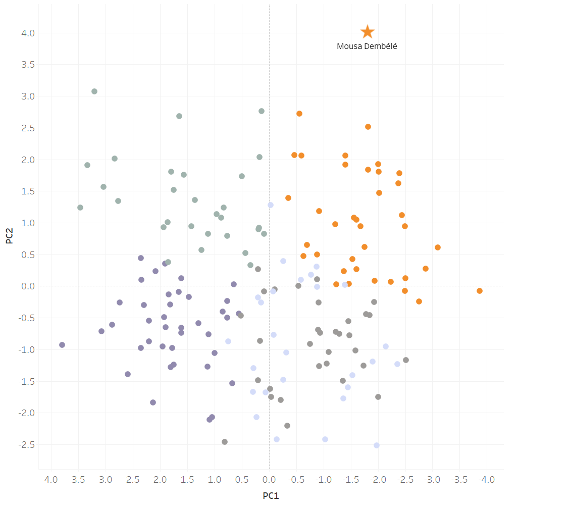
I’ve highlighted Mousa Dembélé as he is the focus of my analysis. Players within Mousa Dembélé’s cluster are what I am interested in, as they are more statistically similar to Dembélé than they are to any other group.
Looking through the players in Dembele’s cluster, there are a host of top class, starting champions league level midfielders. The point of this analysis is to identify potential players that may be a good fit for specific needs. It’s not to replace traditional scouting but rather acts as a starting point for scouts. This can hone in on targets, reducing the potential pool of players that need to be evaluated.
One limitation with the data used was the very wide position filters. The dataset only had midfield, defence, and forwards position identifiers. This meant the midfield pool included a huge range of players from dribbly wingers to defensive midfielders. This has the effect of skewing the clusters somewhat as, intuitively, a winger has a completely different profile to a holding midfielder. More specific position markers would capture more of the range of styles within a position, rather than clustering somewhat more by position as has occurred with this data. More leagues would also improve the scope for analysis in terms of identifying players that are under the radar.
View my final dashboard to browse the results of the analysis:
https://public.tableau.com/views/WhocouldtottenhamhavesignedtoreplaceMousaDemblin2018Clusteranalysis/Dashboard1?:language=en-US&publish=yes&:display_count=n&:origin=viz_share_link