
This blog post will give information on how to use two very important tools: cross tab and transpose. They are each used to pivot the data, meaning it is easy to get their functions confused.
The Cross Tab function is used to orientate data in a table by moving vertical data onto a horizontal axis and summarizing the selected data.
Lets take a look at the Cross Tab tool in action!
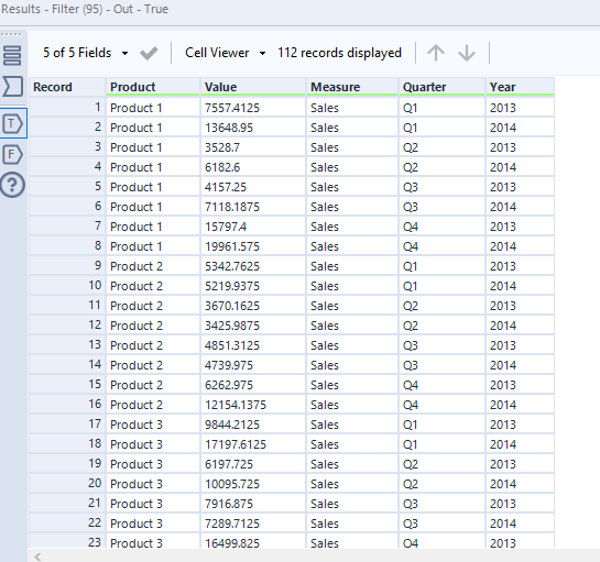
The table below shows various columns, from which we would like to produce two new columns corresponding to the value for each year (2013 and 2014).
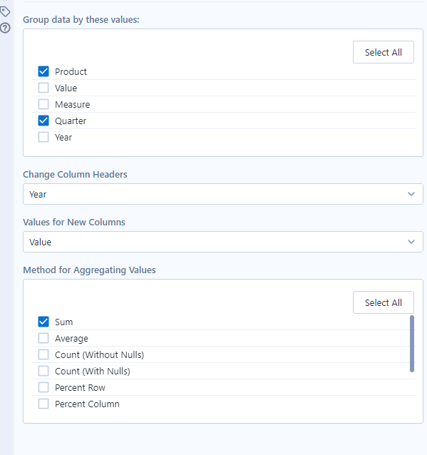
The first step we need to take after establishing this, is to drag the Cross Tab tool onto your workbook. This will produce the options shown below and in this example we would like to group the data by product and quarter, change column header to year and we would like these new columns to show values.
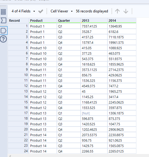
Selecting these options and clicking "Run" will produce the table shown below. This clearly shows the sum of values for each year by product and quarter.
The Transpose tool is used in a very similar way to the Cross Tab tool however it instead pivots the orientation of data in a table by moving horizontal data onto a vertical axis.
An easy way to remember the difference between these tools is by looking at their icons. As shown below, a Cross Tab (on the left) rearranges columns to rows whereas Transpose changes rows to columns.