


In my previous blog, I discussed the SQL query execution order and shared some tips to improve performance (link). However, when working with large datasets or complex queries, those optimizations are sometimes not enough. So, how can we retrieve data faster in those situations?
One powerful solution is using indexes.
In this blog, I’ll cover:
- What an index is
- How to test and compare query performance with and without indexes in MySQL
- How indexes improve query performance
1/ What is the index?
In other programming languages like Python, when working with a DataFrame, we usually see an index column on the left-hand side. This index acts as a unique label to identify each row, and it can be an integer, string, or any hashable type.
However, in SQL, the concept of an index is different.
An index in SQL is not used to identify rows. Instead, it is a data structure that helps the database locate and retrieve data more efficiently.
Without an index, the database has to perform a full table scan, meaning it reads every row from the beginning to the end to find the requested data. With an index, the database can quickly narrow down the search space, significantly improving query performance.
For example, on the last page of the book, you will see an Index page with the list of topics and the page numbers related to that topic. It helps you locate the topic in the book more easily and quickly.
Depending on the RDBMS, indexes can be implemented and supported differently.
2/ How to test and compare query performance with and without indexes in MySQL
I will take an example with the Superstore data source. In this blog, I chose MySQL to query data.
For example, I want to get the total sales of each category in each state. The total sales must be greater than 100,000.
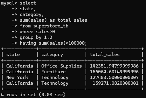
In Fig. 1, I wrote a SQL query to query the data from the superstore_tb table. It took 0.08 seconds to run that query. To understand how this SQL query runs behind the scenes in MySQL, I will use EXPLAIN and set the format in the TREE structure.
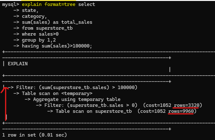
After adding the explain and format=tree at the front of the SQL query (Fig. 2), it will show the result in a tree structure. To track how the flow runs, we will go from the bottom to the top of the tree.
First, it will scan the whole superstore_tb table (9960 rows). Then, it will filter in the sales column to retrieve only values >0 (rows now reduced to 3320). After that, it will aggregate the sum of sales, grouped by state and category columns. Then, it will be stored in a temporary table and scanned again. In the final step, it will filter the sum of sales.
How is the result if I query the data with indexes?
I will create an index with multiple columns on the table superstore_tb. Depending on the platform you are using, the steps to create an index are quite different. For example, in Snowflake, you need to create a Hybrid table before creating an index.
The syntax for creating an index:
CREATE INDEX <index_name> ON <table_name> (column_1, column_2, ...)
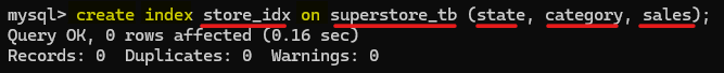
In MySQL, I created a store_idx index on the superstore_tb table for 3 columns: state, category, and sales (Fig. 3). You can also create a single-column index. Note that the order of the column matters in the list.
In my command, the column order will start from the leftmost with state -> category -> sales. SQL will create an index with:
state
state + category
state + category + sales
The question is: How do I know the order of the columns to put in that list?
According to a blog by Franck Pachot, the column order follows:
Equality (=) -> Range (> , <, BETWEEN) -> Sort, Group (ORDER/ GROUP BY) -> multiple ranges (IN)
Based on that order, you can also specify which column to add to the index.
In my SQL query:
select
	state,
	category,
	sum(sales) as total_sales
from superstore_tb
where sales>0
group by state, category
having sum(sales)>100000;
By applying the order above, I have:
- a range sales > 0
- group by state and category
With the rule above, I will put the column in order: sales -> state -> category. However, I put the sales column last. If I put the sales column in the first place, it will run slower because SQL will scan the whole table to check sales >0.
If I move the state, category column in GROUP BY to the first and second place, it will run faster as SQL will scan fewer rows. It will create an index for state and category before checking sales>0.
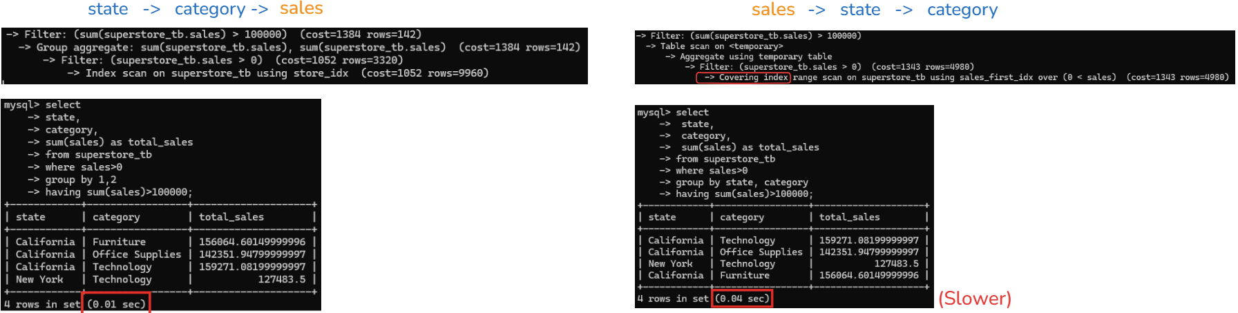
In Fig. 4, I tried to switch the order of the sales column and compared the result. On the left side, the sales column is at the end. On the right-hand side, the sales column is in first place. The running time is different. The left one ran in 0.01 seconds while the right one ran in 0.04 seconds.
With the same SQL query and the column order is different, I ran the SQL query with the EXPLAIN command, and you can see the differences.
On the left-hand side, MySQL uses an index that is ordered by the GROUP BY columns (state, category). Because of this, it can perform aggregation while scanning the index, without creating a temporary table.
On the right-hand side, MySQL uses a covering index that is optimized for filtering on sales >0. However, the index order does not match the GROUP BY columns, so MySQL cannot aggregate. As a result, it must create a temporary table to perform the aggregation and then scan it again to apply the HAVING condition.
Even though the right-hand side uses a covering index and avoids table lookups, it is slower because creating and scanning the temporary table is more expensive.
Another way to see the difference is to show the index when you type the SQL query:
SHOW INDEX from <table_name>
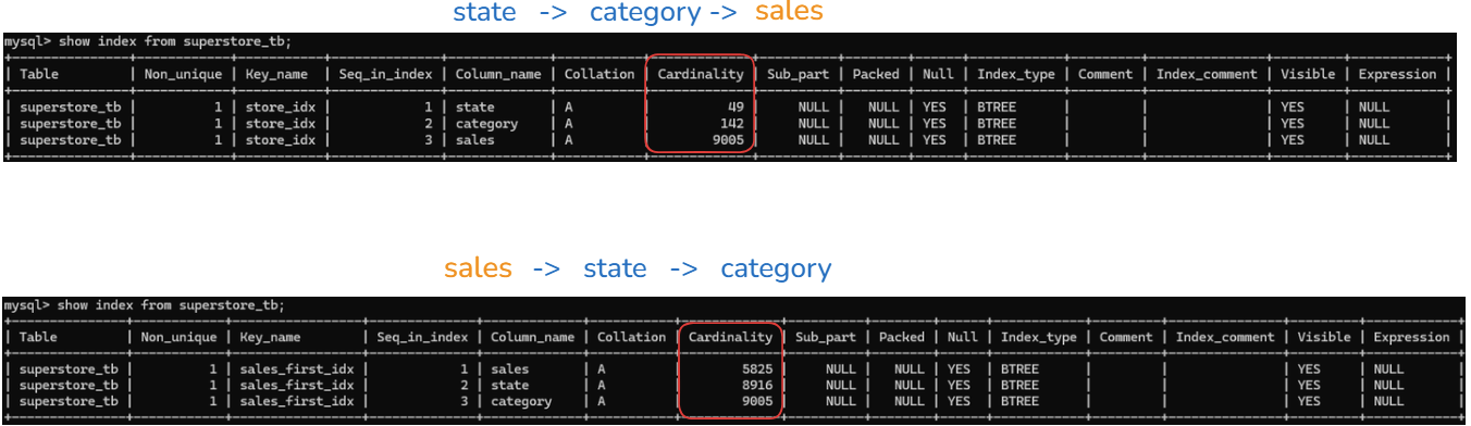
If you look at the Cardinality column from the result table, you will see that the number for each column name is different. However, the last row value in the Cardinality is the same for both tables because it's cumulative.
On the top table, when the sales column is at the last (state -> category -> sales):
- state (cardinality is 49): creating around 49 unique states index
- state + category (cardinality is 142): it combines both state and category to create unique indexes -> 142 values
- state + category + sales (cardinality is 9005): when combining all 3 columns, we have 9005 index values.
On the bottom table, when the sales column is at the front (sales -> state -> category):
- sales (cardinality is 5825): create each row with an index -> 5825 values
- sales + state (cardinality is 8916): when combining sales and states, it increases to 8916 values
- sales + state + category (cardinality is 9005): same value as the top table
The bottom table takes a longer time to run with 5825 indexes at the first scan, while the top table with the state column in group by is only 49.
=> One tip: put the columns in GROUP BY at the front when creating an index, then the range after it.
3/ How indexes improve query performance
If you look at the table in Fig. 5, you will see that the Index_type is BTREE. What is B-TREE?
Documentation page: https://dev.mysql.com/doc/refman/9.6/en/index-btree-hash.html#btree-index-characteristics
In SQL, there are many Index types. They could be B-Tree (mostly), Hash (in Memory table), FULLTEXT (search text), or Spatial index (geo data).
B-Tree stands for Balanced Tree. It was used to implement the index in most data structures in SQL. It contains the root, parent, and child nodes.
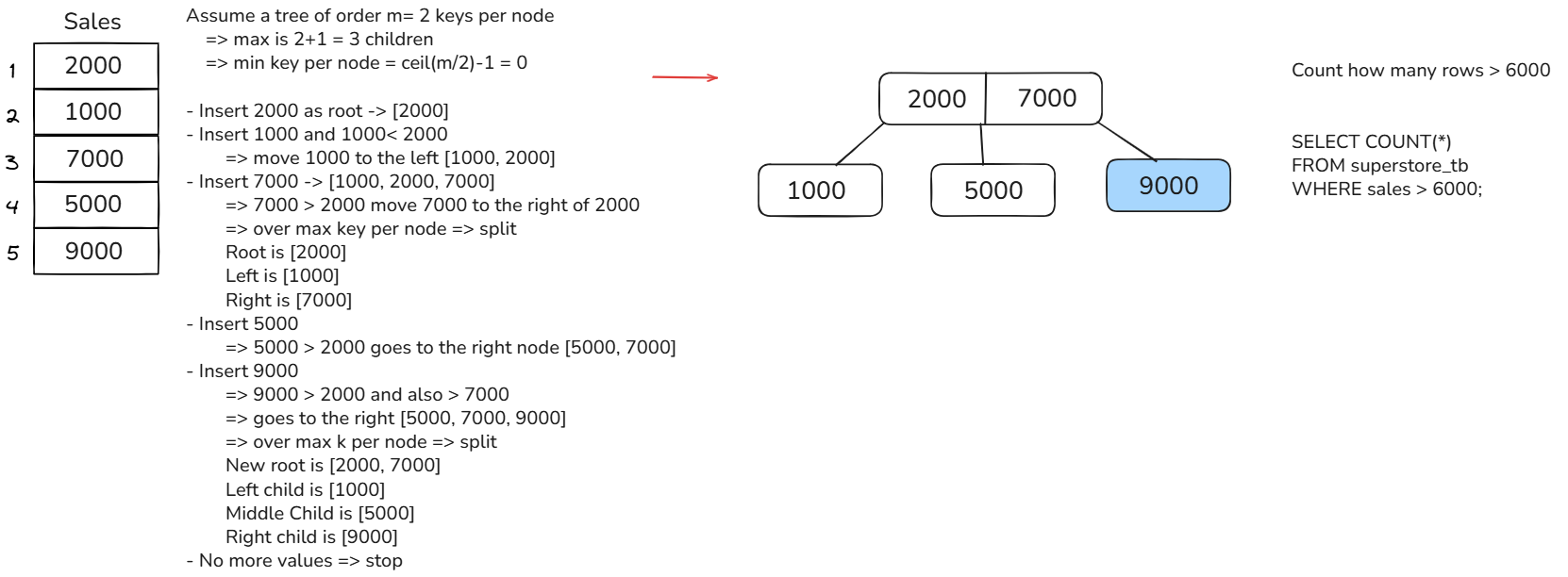
I have an example of a B-Tree in Fig. 6. Assume that I have a column sales with values 2000, 1000, 7000, 5000, and 9000. SQL applied the B-Tree data structure to build a tree.
Then, I have a query to count how many rows have a sales value greater than 6000. By traversing the B-Tree in Fig. 6, it doesn't take a long time to search for values greater than 6000.
From the root, it checks that 6000> 2000 => look at the middle node or right node. Then, 6000 > 5000 (middle node), look at the right node. 6000 < 9000, so returns 1 row. By traversing this tree, SQL doesn't need to scan the whole table.
In this blog, I introduced the concept of indexes in SQL and showed how to create them in MySQL. I also explained why the order of columns matters when creating multi-column indexes and how this can affect query performance. Finally, I focused on one type of index, the B-Tree, and illustrated how it works to retrieve data efficiently.
I hope this blog helps you understand how indexes work and how to leverage them to retrieve data more quickly in your SQL queries.